Human brain theory

4.3.  Modules with spatial signal propagation 

4.3.1 The brightness module with spatial signal propagation

 

The brightness module with spatial spread developed from the brightness module with lateral spread through a growth in the thickness of the outpouch layer - combined with an increase in the number of output neurons. These were now spatially distributed in the outpouch layer. Thus, in addition to the x-coordinate and the y-coordinate, the z-coordinate was added for the height of a neuron in this layer.

We should bear in mind that in many vertebrates, thickness growth probably occurred first, while lateral growth started later.

In this monograph, we have first described the consequences of thickness growth and, in the case of the orientation columns, we have initially excluded this thickness growth. Otherwise the mathematical apparatus would have become completely opaque. Now, however, we extend the concept of the previous chapter to include thickness growth. In addition, we process the brightnesses in the extended module.

Thus, instead of the previous four input neurons, we now need eight. Four input neurons from magnocellular ganglion cells provide the dark-on input to layer 4-dark-on. Above it is layer 3-dark-on. Above it is layer 4-Light-On. This is where the signals from the four light-on type ganglion cells arrive.

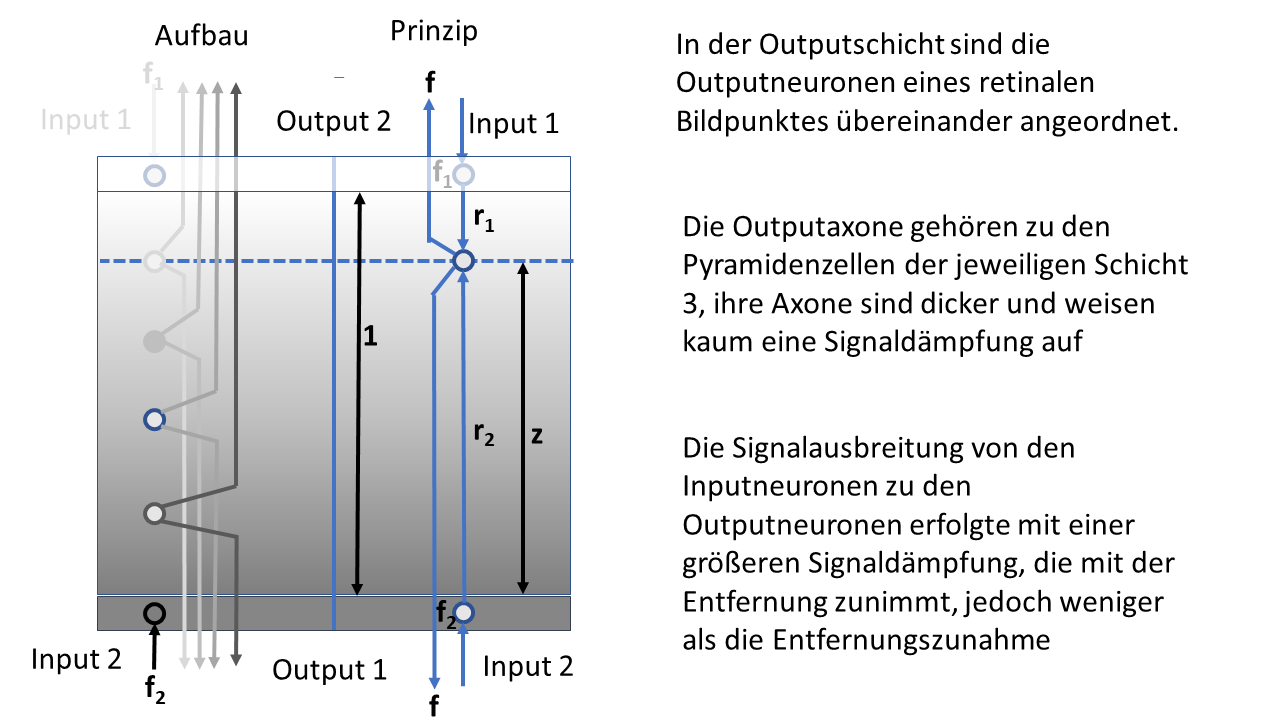
Figure 30: Brightness module with spatial signal propagation

In the figure above, the module can be seen in cross-section, its lateral extension is not shown here. Important for the later considerations is the height z of the output neuron whose excitation we will calculate.

In the chapter on the brightness modulus with lateral signal propagation, we related the firing rate of a magnocellular ganglion cell to the chordal length s. The firing rate of a magnocellular ganglion cell is determined by the chordal length s. A dark, inclined straight line with an angle of attack α intersects the circle formed by the receptive field of the ganglion cell and leads to darkening there. The dark-on type ganglion cell reacts to this darkening by increasing the firing rate. We assumed that the firing rate would be equal to the square of the chord length. A possible proportionality factor falls out when differentiating.

We arrange the circle in the x-y plane as shown in the following figure.

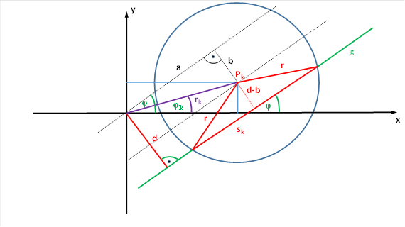
Figure 31: Calculation of the chord length for a receptive field of a ganglion cell

Then, for the square of the chord length _{sk the} equation results

This has already been proven in chapter 4.2.3.

We now examine the chord length squares for four retinal ganglion cells in the following arrangement, which was already used in chapter 4.2.4.

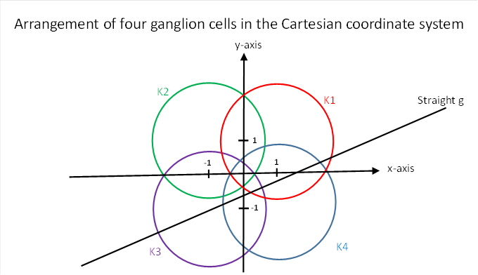
Figure 32: Arrangement of four ganglion cells in the Cartesian coordinate system

For the squares of the chord lengths, which are ultimately used as the firing rate of the ganglion cells, the formulae apply (as derived in 4.2.2.)

We can simplify the expressions in the angular functions. Because, according to our assumption, the firing rate of each ganglion cell corresponds to the square of the chord length, the following equations apply to the four firing rates:

Reminder: r is the radius of the receptive fields of the four magnocellular ganglion cells, i.e. the four circles intersected by the straight line g.

These firing rate formulae apply when a black line against a white background intersects the receptive fields of the four dark-on-type ganglion cells involved.

In a system where the magnocellular ganglion cells can also evaluate luminosities, the firing rate for a black straight line will take on exactly the values of the squared chord length.

However, if the straight line is not black but grey, the ganglion cell (of the dark-on type) will be less excited. A correction factor will be needed which, as the grey value of the straight line increases, decreases the firing rate so that it becomes less than the chord length square. We decide to use an exponential approach, which has already proved successful with the motor divergence module.

Let h be a quantity from the interval <-1,+1>. Let us call h the relative brightness - it can be interpreted as a positive or negative percentage. Thus white corresponds to brightness 1, black to brightness -1.

If fs is the firing rate of a dark-on ganglion cell when there is a black object in the receptive field of this cell and f(h) is the firing rate when the object is not black but has the grey value h, let the following hold:

We now have to consider in the four firing rates of our ganglion cells the relative brightness u of the line intersecting the receptive fields. Thus we obtain the formulae

So that in future we can distinguish the firing rates of the dark-on ganglion cells and the light-on ganglion cells, we choose the index D for the above dark-on ganglion cells, it is to represent the word dark. Then the following applies to our four firing rates:

The firing rates of the bright-on ganglion cells, when a bright line with brightness h (the grey value h) appears against a black background, satisfy the formulae

Thus, we now have the firing rates of four ganglion cells of the dark-on type and four of the light-on type, as well as the associated firing rates. Of these eight ganglion cells, four now project into the magnocellular sublayer 4-Dark-On, the remaining four into layer 4-Light-On.

Let the topological arrangement be given. We have a total of four adjacent eye dominance columns from the same eye. This creates a cube. Its four upper corners receive the retinal light-on input. The lower corners receive the dark-on input.

Each individual firing rate is to be provided with the correction factor for brightness h in the case of a dark-on ganglion cell, if the line does not have the colour black but the relative brightness h. The same applies to the light-on ganglion cells. We have already incorporated these correction factors into the eight firing rates. We first consider the four dark-on input neurons. They may be arranged exactly as in the previous chapter

.

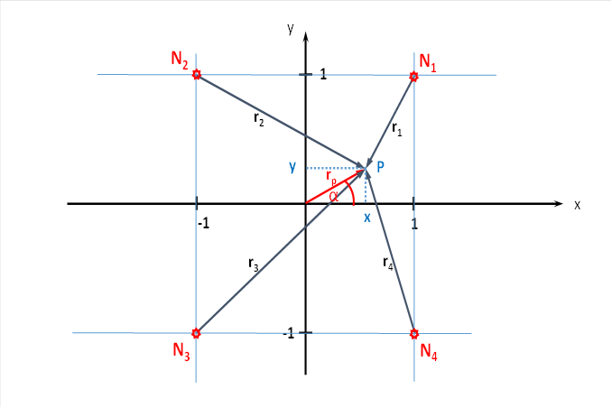
Figure 33: Four cortical output neurons in the brightness module with spatial signal propagation

We had already derived a formula for the firing rate of the neuron at point P:

It results this way because a distance-dependent damping occurs, which increases exponentially with the square of the distance travelled. Thus the rate of fire will decrease exponentially with the square of the distance, hence the negative exponent in the e-function.

Now we have to consider that the divergence module is spatial. Besides the width x and the length y, there is a height z for each neuron of the layer S3-Dark-On.

We consider the output neuron that has the already known coordinates x and y in the width and length, and that has the height z at the same time. To do this, we fold the x-y plane from the illustration into the horizontal plane. Then the output neuron is located at the point P(x,y,z) exactly vertically above the point P of the above figure.

If we connect the point P(x,y,z) with the lower corners of the cube, i.e. with N1 to N4, we get four new vectors t1 to t4. They connect the point P(x,y,z) with the lower corners of the cube and indicate the length of the distance that the neuronal excitation has to cover from the corners of the cube to the point P(x,y,z).

Then the excitation _fu arriving from the four lower corners at the point p(x, y, z) is equal to

In the sketch, you can see the change when the excitation from the four output neurons spreads out spatially and reaches the point P(x,y,z), whose height above the x-y plane is equal to Z.

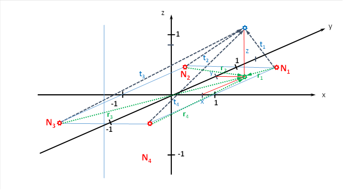
Figure 34: Derivation of the length of the radius vectors for the brightness module with spatial signal propagation

 

From neuron N1 (shown in red), the new radius vector t1 runs to the output neuron (blue) with height z (red). It forms the hypotenuse of a right-angled triangle whose kathets are formed by r1 and z. According to Pythagoras, the following therefore applies

The following applies analogously for the other three new radius vectors

We can insert these new radius vectors into our formula for the output neuron.

We can exclude the common component that occurs in all four summands and draw it as a factor in front of the sum.

This is the formula for the excitation that the output neuron P(x,y,z) receives from the four lower input neurons. The excitation is obtained for spatial excitation propagation by choosing the excitation for propagation in the x-y plane and multiplying it by the factor  multiply.

We now change the names for the four input excitations f1 to f4 in retrospect. The reason is simple: they are the input of the four dark-on neurons from the retina. Therefore, we replace the symbol f with the symbol fD.

The firing rates fD = fD(h) are obtained by multiplying by the correction factor e-u, we can write this as a proportionality factor in front of the sum. Therefore

This excitation contribution is made by the lower four dark-on neurons when the inclined straight line that intersects their receptive fields has brightness u.

This excitation part consists of two factors.

The first factor takes into account the distance z of the output neuron at the point P(y,x,z) from the x-y plane and the brightness of the straight line intersecting the receptive fields of the four on-type neurons of the retina.

The second factor

is exactly the firing rate of the brightness module with lateral signal propagation of the dark-on type, which we have already derived in chapter 4.2.2.

Now we have to consider that our output neuron not only receives input from the lower corners of the cube with edge length 1, but also from the four upper corners.

Here, however, the distance of the output neuron (blue) to the upper surface of the cube is exactly 1-z, because our cube should have an edge length of 1.

Therefore, our formula for the input from above is obtained by replacing the distance z in the formula for fD with the new distance 1-z and instead of fD we now use fH. This is because the top four superior neurons receive from the retina the light-ON signals of those magnocellular ganglion cells that belong to our four retinal points. Each retinal point has a dark-on signal and a light-on signal.

Thus our output neuron receives the following excitation from the upper four neurons:

The influence of the signal propagation in the z-direction (signal attenuation) is taken into account by the first factor, the contribution of the signal attenuation in the x-y-plane by the radius vectors r1 to rk.

However, in our extended model, the bright-on ganglion cells do not receive the brightness of a white straight line in front of a black background, but of a straight line with brightness u. Therefore, we have to consider the correction factor e+u for brightness for all firing rates.

Here the influence of the signal propagation in the z-direction (signal attenuation) is taken into account by the first factor, the contribution of the signal attenuation in the x-y-plane by the radius vectors r1 to rk.

This excitation part also consists of two factors:

The second excitation part

again agrees exactly with the firing rate of the brightness module with lateral signal propagation of the dark-on type, which we have already derived in chapter 4.2.2. The influence of the brightness is caused by u, the light-on type is caused by the positive sign of the brightness. Here the off-type had a negative sign.

We consider that the output neuron receives both the contribution of the lower input neurons, but also the contribution of the upper input neurons. Its total excitation therefore consists of a sum.

Inserting the two partial excitations gives the final firing rate of the output neuron in the spatial divergence module.

The following applies

 

We combine the first two factors into a new function, which we call the height function H of the visual divergence module with spatial signal superposition.

Then we can write the excitation of any output neuron within the cube we are considering as a function product.

The function f(x,y) is the excitation function we encountered in the visual divergence module with lateral signal propagation in the case of the magnocellular input.

We now ask for the location of the output neuron in the cube under consideration that has the strongest excitation.

The strict concavity of excitation propagation for a single neuron within a convex environment where the Hessian matrix is negative definite guarantees that the superposition of multiple excitations from different output neurons within the superposition of these environments results in a global maximum.

For the calculation, in the case of spatial signal propagation, the partial derivative to x, to y and additionally to z must be formed and set equal to zero.

Here it proves to be a tremendous advantage that the excitation function f consists of the two factors H(z,u) and E(x,y). The first factor contains only the variables z and u. The variable u stands for the current brightness and can be regarded as a preliminary constant. The variable z indicates the height of an output neuron in the cube.

The second factor is a function that depends only on x and y and is identical to the excitation function of the brightness module with lateral signal propagation. Here we have already calculated the derivatives to x and y and set them to zero. Thus we have derived the formulae for the angle of rise and the zero point distance of an inclined straight line. Exactly these conditions for the x-coordinate and the y-coordinate and the requirements for the associated phase angle and the radius vector in the x-y plane also apply in the module with spatial propagation.

The height coordinate of the maximum neuron is given by the function H(z,u). Here, the brightness u determines the height coordinate z.

This must be determined by forming and setting to zero the derivative of the function H(z,u) with respect to z. The function E(x,y) appears in the excitation function as a constant factor because this function does not contain the variable z at all. The constant factor is divided out when zeroing and therefore falls out.

So all we have to do is calculate the derivative of the function H(z,u) with respect to z and set it equal to zero to find the height z of the maximum neuron in the cube.

We calculate the derivative:

Transform results in

 

 

 

With this equation we can determine what brightness value u the straight line must have so that the neuron with height z within the cube achieves the maximum excitation among all neurons of this cube.

This neuron is most excited among all the neurons in the cube when the angle of attack φ of the inclined straight line in the field of view satisfies the condition,

which we had already derived for the brightness module with lateral signal transmission:

 

If the brightness of the straight line changes without changing its angle and position, then only the height z of the maximally excited neuron changes, while the coordinates x and y remain unchanged.

With the thickness growth of the magnocellular outpouch layer of class 3 of the cortex, again a new modality emerged: brightness value of line elements.

Whereas in the single-layer neuron layer only black or white line elements could be analysed in terms of their orientation angle, the new modality could detect the brightness of these line elements according to grey levels. Because new modalities split up in the course of evolution and drive their own separate secondary cortex areas, as many retinal images now arose in the secondary visual cortex as there were grey levels. But because each retinal image was already broken down into separate images for the different angular ranges, there was a separate retinal image for the combination of each grey level with each detectable angular interval.

So with 20 grey levels and 30 angular intervals, there were a total of 600 retinal images in the secondary cortex. These were not wildly mixed. Markers ensured that, for example, in the longitudinal direction the retinal images were sorted according to ascending orientation directions of the line elements, while in the width the sorting was done according to ascending brightness values (grey tone sorting).

This seems very real to me, because it allowed each retinal image to respond to emerging signals. A centroid module for each of these many retinal images calculated the location of the signal centroid and sent signals to the eye muscles that caused them to centre on the signal centroid.

However, since only very few of the countless retinal images were active at any one time (a line could in principle only produce one angular value on a retinal point - crossing lines a maximum of two,...), neuronal activity constantly shifted from one retinal image to the next when something changed. Therefore, activity centres in the secondary visual cortex move back and forth when watching a film, for example.

Important comment:

As the author, I have made some basic assumptions in this monograph. For example, the assumption that the excitation of a neuron spreads in the spatial divergence moduli according to the formula

where f(0,0,0) is the firing rate at the coordinate origin, where the input neuron is also located. The output neuron, on the other hand, is located at the point P(x,y,z) and has the distance r from the coordinate origin. As a physicist, the formula

would have been much preferred. But the approach I have chosen ensures that the excitation of a neuron in a cube that takes its input from the eight corners, from which the lower neurons receive the inverse signal of the upper ones, always leads to the formation of orientation columns when an inclined straight line appears in the receptive field. Here, one can cut the cube into small horizontal slices and notice the following in amazement:

In each of the horizontal discs there is exactly one excitation maximum. As long as the angle of attack and the position of the straight lines remain unchanged, the locations with the maximum excitation in each of these thin discs lie exactly above each other.

Any neurologist who pokes vertically into such a neuron cube with a fine measuring probe will (if he catches a neuron) receive a neuronal signal. If he moves an inclined straight line through the image field parallel to himself, this neuron will fire maximally at a certain position of the straight line, if this straight line has the most favourable setting angle for this neuron. So you have to patiently change the angle of attack and the position of the straight line until this one neuron fires maximally.

If you now move the fine measuring probe deeper, you tap into a deeper layer of the cube. Surprisingly, the neuron there is also maximally excited, because the neighbouring neurons at the same height fire less strongly. This is why the term orientation column was coined. All neurons in the column are very strongly excited at a certain angle of attack characteristic of this column, but only one among them is always the most strongly excited.

If I had used the third power in the transfer function f(x,y,z) instead of the second power of the distance, the excitation maxima in the layers of the neuron cube at different heights would no longer have been exactly superimposed. The differential of the function would not be decomposable into two factors, one of which only has the coordinates x and y of the plane, while the second factor only includes the height coordinate z. Only then does the excitation in a plane parallel to the x-y axis always have its global maximum at the same point if the angle of attack of the straight line and its position are constant.

This experimentally confirmed finding led me to the mathematical approach of setting the damping of neuronal excitations during propagation in space with the second power of the distance from the excitation source. So it was not arbitrariness to gain simpler formulas, but the desire to choose the formulas that fit experimentally proven facts. Reality should be the yardstick for the choice of the neuronal transfer function.

The measuring neurologists can now be given a new measurement assignment: Prove by measurement that the excitation within the same orientation column depends on the height and that the height z in the magnocellular part of the column encodes the brightness of the straight line (its grey tone). For each grey tone of the straight line, exactly one neuron is maximally excited in this column. Its height depends directly on the grey value of the straight line.

In the parvocellular part of the column, prove the following: Within an orientation column associated with an angle of attack and a position of the straight line in the field of view, the height of the maximally excited neuron depends on the colour of the line. Each colour is uniquely associated with the depth of the puncture with the probe.

The orientation column can be divided into colour layers in such a way that they are arranged horizontally. The colour detected by the neurons of this layer is identical in the entire horizontal layer. The neuron height in the parvocellular cortex layer V1 is assigned to exactly one colour as long as one moves within the colour module.

And because the position of a colour in height was determined via the first derivative, the law of colour constancy applies. Constant factors such as brightness fall under the table when differentiating, their influence disappears completely.

 

3.3.2.   The colour module with spatial signal propagation

 

After explaining the brightness module with spatial signal propagation, it is time to put the module concept to the test.

It was claimed by me that a change of modality has no influence on the work of a brain module. We will now show this.

If one replaces the magnocellular visual input with the parvocellular one in the brightness module with spatial spread, all formulae remain the same. The firing rates here no longer reflect the detection of a straight line with a given grey level, but the grey level is replaced by the colour saturation. The bright-on ganglion cell now reacts to red light in the red/green module. It is of the On type. The stronger the red component of the light - and light is usually a mixture of colours - the stronger the red-on neuron fires. By contrast, it is inhibited by green light components.

The dark-on ganglion cell is replaced by the green-on ganglion cell. The higher the green component of the light, the stronger it fires.

Let u again be a relative quantity that evaluates the relative red component in relation to the green component and can assume values from -1 to +1. The value u = 1 corresponds to the colour value red, the value -1 to the colour value green. The value u = 0 then corresponds to the colour value yellow according to the laws of colour mixing.

If fH is the firing rate of the red-on ganglion cell and fD is the firing rate of the green-on ganglion cell, which is also a red-off ganglion cell, the following equations may apply:

Thus, the input does not differ significantly from the input into the brightness module with spatial transmission.

If a straight line with the colour value u > 0 now appears in the receptive field of the ganglion cell, while the background has the complementary colour (to which the ganglion cell reacts almost not at all), the firing rate again grows quadratically with the chord length. It was the same in the brightness module.

Therefore, the output behaviour of the neurons of a cube whose lower corners receive the on-input from the green-sensitive and squared retinal ganglion cells, and whose upper corners receive the associated retinal input from the red-sensitive ganglion cells of the same retinal points, does not differ mathematically in any way from the brightness module with spatial signal propagation.

The red input takes the place of the light input. The place of the dark on-input is taken by the green on-input.

And since we now know that the red-green input in the cortex reaches the parvocellular layers S4-green and S4-red, between which lies the output layer S4-green, but whose neurons can receive both the green input from the lower input layer and the red input from the upper layer, the excitation from these two types of colour receptors spreads and overlaps in the layer S3-green. This is because a total of 8 input neurons deliver their signals to this cube. Exactly the same physical and mathematical laws apply to it as to the light-dark module.

Therefore, there are orientation columns again in the green-red module with spatial signal propagation. These react to the angle of inclination of a straight line according to the same formulae. And since the neurons in both the light-dark module and the green-red module are arranged retinotopically, input neurons of one and the same retinal site in the visual cortex cortex also lie exactly on top of each other. Therefore, a red/green orientation column, when maximally excited, will require the same angle φ and the same zero point distance d as the orientation column of the light/dark module.

And the same applies to the colour combinations blue-green and red-blue.

The maximum excitation at a given angle φ and a zero point distance d of the inclined straight line depends only on the x-coordinate and the y-coordinate in all visual modules of the primary visual cortex cortex, regardless of the layer system. The module cubes for brightness and colours are simply stacked on top of each other. Therefore, an orientation column goes completely through from the top to the bottom layer and consists of an upper quarter for the colour mixture blue-red, below that a quarter for the colour mixture green-red, again below that a quarter for the colour mixture red-blue and at the very bottom a quarter for the module light-dark. The x-y coordinates of the master-excited neurons in this neuron cuboid determine the angle of ascent and the zero point distance of an inclined straight line, the height, on the other hand, determines the colour and the brightness. In each of the four modules there is - if a visual stimulus is offered - exactly one maximally excited neuron. However, the other neurons of the square are also excited, but the most excited neuron in a module forms the centre of excitation.

When the output leaves the superposition layer, lateral neighbour inhibition occurs and suppresses the weaker signals so that the neurons with the highest firing rate prevail. Their output reaches further brain areas.

Since the retina projects by means of many thousands or hundreds of thousands of ganglion cells of different modalities (light/dark, colour-on/colour-off) into the primary visual cortex, it forms (in humans) a signal image of the visual environment in the four visual submodalities. Points of the same colour lie at the same level, the neurons there fire when this colour is detected - but only if line elements have the required directional property.

If there are no inclined straight lines, i.e. no contours, because there is a surface of the same brightness or the same colour, then in this case those neurons fire in the modules that have the x-y coordinates zero in the associated cube or cuboid. If neurons with the coordinates x = 0 and y = 0 fire, there is no line in the receptive fields of the signal-providing retinal cells. Then coloured areas are simply perceived and their brightness determined. This signal path is used for object analysis, while the other orientation columns analysed the directions of line elements of different colours. Because they represented different modalities, their paths separated in the secondary cortex. And when the signals found their way to the dopaminergic midpoint centre, which always had to take all signals into account, the way was prepared for motion detection. On the long way from the first, cortical segment to the dopaminergic substantia nigra in the seventh segment, the visual signals had to suffer a time delay and became past signals. Now the present and the (recent) past were available to the brain in signal form. The back-projection of the dopaminergic mean nucleus to the cortex thus exhibited a time delay. This type of signal was a new modality: the past. This was only a few milliseconds back, but could be used in a new module for motion detection. This new module was the basal ganglia. The next chapter is dedicated to them.

Anyone who has understood how the superposition modules work with spatial signal propagation knows how the primary cortex works in principle. It does not matter whether the modality is visual, motor, tactile, pain, electrosensory, lateral line or any other modality.

Nevertheless, there is downstream signal processing for all these modules, the result of which has an effect back on these primary cortex areas. Only in this way is it possible for neurons in the primary sensory areas to react to movements. This reaction is achieved by downstream signal processing in delay modules. These are located in the brain of vertebrates in the basal ganglia system.

At this point I would like to gratefully point out that I owe all my knowledge about the basal ganglia and their cytoarchitectonic structure to Prof. Dr. Rolf Kötter. He himself was a student of Prof. Karl Zilles, whose wonderful works gave me easy access to the human nervous system. Especially his very detailed descriptions and illustrations of the most diverse signalling pathways in the brain gave me the ability to imagine the human brain in all its substructures in my mind and to analyse it. The work of his doctoral students was always a treasure trove of new insights for me. In addition, I owe Prof. Gerhard Roth the insights into the development of the brain during the many millions of years of evolution that once began with simple clusters of cells.